Decided to play with the latest version of Gephi by creating a new musician network, and wound up creating six using MusicBrainz data. This was a fun project and will be followed by additional work covering more great jazz musicians. Here’s a quick screenshot of one of the graphs showing the artist, album releases, and songs associated with those releases:

I’ll post the links to each network below and then take a walk through the creation process. Note that the graphs are all interactive, with panning, zooming, edge removal, and other features all available. More on those features later in the post. Here are the links to each network graph:
Note that there are at least two major omissions among saxophonists – Charlie Parker and John Coltrane, and of course some other notable names. I’ll plan to address those omissions in a future post.
To create each of these graphs I followed a simple set of steps and then used the same settings to create graphs with a consistent look & feel. The goal is to have users focus on the structure and content of the network as opposed to having to deal with changing shapes, sizes, and colors. Perhaps I’ll alter this for different instruments – piano or trumpet, for example may have a different color palette. For now, the color palette I have used conveys an appropriately jazzy aura, with the dark background and contrasting pastel-like node colors and subtle gray edges connecting the nodes.
The data for this project is sourced from the impressive MusicBrainz database. Note that MusicBrainz data covers many genres beyond jazz, but for my current purposes the focus is on jazz. I have created a local version of the data using DBeaver for writing and running SQL queries to retrieve data for ingestion by Gephi. DBeaver is a great solution for me – all of my other databases are in MySQL, while the MusicBrainz data is in PostgreSQL format. No problem, as DBeaver can handle both types (as well as many other data formats) with ease.
Here’s an example of the code used for node creation for Sonny Rollins:
SELECT a.*
FROM
((SELECT CONCAT(ac.name, ' (Artist)') AS id, ac.name AS name, ac.name AS label, 'Artist' AS type, 50 AS size
FROM public.artist_credit ac
WHERE ac.id = 21832)
UNION ALL
(SELECT CONCAT(r.name, ' (Release)') AS id, r.name AS name, r.name AS label, 'Release' AS type, COUNT(DISTINCT rl.release) AS size
FROM public.release r
INNER JOIN public.artist_credit ac
ON r.artist_credit = ac.id
INNER JOIN public.medium m
ON r.id = m.release
INNER JOIN public.medium_format mf
ON m.format = mf.id
INNER JOIN public.release_label rl
ON r.id = rl.release
INNER JOIN public.label l
ON rl.label = l.id
WHERE r.artist_credit = 21832
GROUP BY r.name
)
UNION ALL
(SELECT CONCAT(ta.name, ' (Song)') AS id, ta.name AS name, ta.name AS label, 'Song' AS type, COUNT(DISTINCT rl.release)
AS Size
FROM public.release r
INNER JOIN public.artist_credit ac
ON r.artist_credit = ac.id
INNER JOIN public.medium m
ON r.id = m.release
INNER JOIN public.medium_format mf
ON m.format = mf.id
INNER JOIN public.release_label rl
ON r.id = rl.release
INNER JOIN public.label l
ON rl.label = l.id
INNER JOIN public.track t
ON m.id = t.medium
INNER JOIN public.track_aggregate ta
ON t.name = ta.name
WHERE r.artist_credit = 21832
GROUP BY ta.name
)) a
While the code may appear complex, it’s goal is simple – retrieve all releases and songs for the artist Sonny Rollins, who has the ‘21832’ id. This code creates nodes for the artist (first section), all releases (second section) and all songs (third section). It uses the UNION ALL statement to combine the three sections into a single output file.
We then run similar code to create an edges source file:
SELECT a.*
FROM
((SELECT CONCAT(ac.name, ' (Artist)') AS source, CONCAT(r.name, ' (Release)') AS Target, 'Artist' AS source_type, 'Release' AS target_type
FROM public.artist_credit ac
INNER JOIN public.release r
ON ac.id = r.artist_credit
INNER JOIN public.release_label rl
ON r.id = rl.release
WHERE ac.id = 21832)
UNION ALL
(SELECT CONCAT(r.name, ' (Release)') AS Source, CONCAT(ta.name, ' (Song)') AS Target, 'Release' AS source_type, 'Song' AS target_type
FROM public.release r
INNER JOIN public.release_label rl
ON r.id = rl.release
INNER JOIN public.medium m
ON r.id = m.release
INNER JOIN public.track t
ON m.id = t.medium
INNER JOIN public.track_aggregate ta
ON t.name = ta.name
WHERE r.artist_credit = 21832)) a
GROUP BY a.source, a.target, a.source_type, a.target_type
This output will instruct Gephi to use the artist as a source node and all releases as target nodes (first section) and then to use all releases as source nodes with songs as target nodes. Think of this as a hierarchy of Artist –> Releases –> Songs where individual songs are associated with the release they appeared on. Of course, in jazz, many of the most popular songs will appear connected to multiple releases, ultimately making for a more interesting graph.
Now that we have created the source files, let’s shift to Gephi to see how we use them.
Gephi allows us to pull in spreadsheet files as long as they meet certain criteria. Node files should have a name, label, id, and preferably a size attribute, although this can be created within Gephi based on the data. Edge files must have source and target fields, and ideally a weight value corresponding to the strength of network connections.
Here’s our data after ingestion, starting with the nodes:
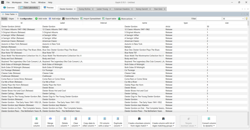
I forget to mention the usefulness of having a ‘type’ column; this will make it simple to set node colors in Gephi. Now the edges file:

You can see the source and target values, which are critical to how the graph will be displayed. Our edge weights are all set to 1 in this network, but frequently we will have varying numbers to indicate stronger versus weaker connections.
Here’s our completed graph in Gephi, after using a number of settings:
- Setting the node colors by type in the Partition tab
- Sizing the nodes in the Ranking tab
- Choosing a layout algorithm – Force Atlas 2 is a popular choice
- Scaling the graph to an appropriate size
- Preventing overlap of nodes
This process can be very iterative, playing with different settings until you are pleased with the results. For graphs like this with hundreds of nodes, different options can be tried very quickly.

The next step is to export the underlying data as a graph file – .gexf is my choice for the web template I use. Here’s a small subset of the Dexter Gordon .gexf file showing the name, type, and size associated with each node.

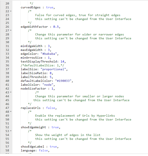
Next, we can update settings in the config.js file; These will adjust the display parameters for the nodes and edges; note that there is also a .css (Cascading Style Sheet) file where many more modifications can be made.
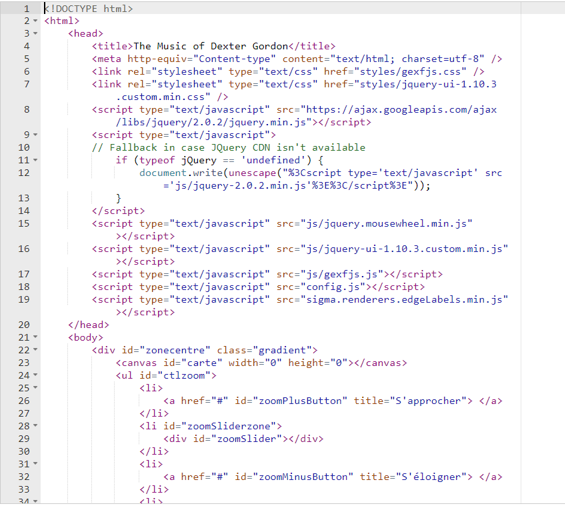
Finally, we have the index.html file that contains links to several scripts as well as the config file. This is where we can also add a title and small bits of information about the graph content.
I’ll be creating additional network graphs using this same end to end approach. The process becomes easier once the code has been tested and validated, and the settings have been standardized in Gephi and the resulting output files; much of the effort will simply involve copying and pasting existing settings. Watch this space for new graphs, and thanks for reading!
